Submarine Targeting Computer

In this post we want to explore how data acquisition for the torpedo data computer can be supported with basic information from the periscope.

Typical view of a target from the attack periscope

Angle on bow

It is easy to see the percieved length is composed of the projection
of the length and beam onto the observer plane.
Hence

(1) $\begin{equation*} \sin(\alpha)l + \cos(\alpha)b = p \end{equation*}$

where $l$ is the lenght, $b$ the beam and $p$ the percieved length.
It is possible to find four different $\alpha$ ‘s for a specific $p$ (As we will see later for some $p$ there are actually eight solutions). If $\alpha$ is a solution $\pi - \alpha, \pi + \alpha, 2 \pi - \alpha$ are also solutions. The correct one can be determined by recognizing the aspect of the target, the cartesian product of ([starboard, port], [hot, cold]), where ‘starboard’ means $\alpha \in [0, \pi]$ and ‘hot’ means $\alpha \in [\pi/2, 3\pi/2]$ and the others the according complement to each other. So each specific product coresponds to one of the quadrants and each quadrant has one or two solution for $\alpha$ .
We can solve (1) for $\alpha$ with some basic math.

(2) $\begin{equation*} |\sin(\alpha)l| + |\cos(\alpha)b| = p \end{equation*}$

or if we limit $\alpha \in [0, \pi/2]$

(3) $\begin{equation*} \sin(\alpha)l + \cos(\alpha)b = p \end{equation*}$

With a larger $\frac{l}{b}$ ratio the overlapping interval becomes smaller. A typical value for a ship is at least 5.

With $\sin(\alpha) = \dfrac{\tan(\alpha)}{\sqrt{1+\tan^2(\alpha)}}$ and with $\cos(\alpha) = \dfrac{1}{\sqrt{1+\tan^2(\alpha)}}$ for $\alpha \in [0, \pi[$

(4) $\begin{equation*} \dfrac{l \tan(\alpha)}{\sqrt{1+\tan^2(\alpha)}} + \dfrac{b}{\sqrt{1+\tan^2(\alpha)}} = p \end{equation*}$

(5) $\begin{equation*} \l \tan(\alpha) + b = p\sqrt{1+\tan^2(\alpha)} \end{equation*}$

Squarring both sides results in

(6) $\begin{equation*} l^2 \tan^2(\alpha) + 2 lb \tan(\alpha) + b^2 = p^2(1+\tan^2(\alpha)). \end{equation*}$

This turns in a quadratic equation for $\tan(\alpha)$ .

(7) $\begin{equation*} (l^2 - p^2) \tan^2(\alpha) + 2 lb \tan(\alpha) + b^2 - p^2 = 0 \end{equation*}$

which can be solved with infamous quadratic formula $x_{1/2} = \dfrac{-b \pm \sqrt{b^2 - 4ac}}{2a}$ for $ax^2 + bx +c =0$ .

(8) $\begin{multline*} \tan(\alpha)_{1/2} = \dfrac{-2lb \pm \sqrt{4l^2b^2 - a(l^2-p^2)(b^2-p^2)}}{2(l^2-p^2)} = \dfrac{-2lb \pm 2\sqrt{l^2p^2 + p^2b^2 - p^4}}{2(l^2-p^2)} \\ = \dfrac{-lb \pm p\sqrt{l^2 + b^2 - p^2}}{l^2-p^2} \end{multline*}$

Now we need to figure out which solution is valid in which interval. For that we determin the limits.

(9) $\begin{equation*} \alpha_1=\arctan \left(\dfrac{-lb + p\sqrt{l^2 + b^2 - p^2}}{l^2-p^2} \right) \end{equation*}$

(10) $\begin{equation*} \lim_{p\to b} \alpha_1(p) = 0 \end{equation*}$

This is the correct result for $p=b$ .

(11) $\begin{multline*} \lim_{p\to l} \alpha_1(p) = \lim_{p\to l} \arctan \left(\dfrac{-lb + p\sqrt{l^2 + b^2 - p^2}}{l^2-p^2} \right) \\ {\overset{\text{l'Hosptial}}=} \lim_{p\to l} \arctan \left(\dfrac{\sqrt{l^2 + b^2 - p^2} - \frac{p^2}{\sqrt{l^2 + b^2 - p^2} }}{-2p} \right) = \arctan \left(\dfrac{l^2 - b^2}{2lb} \right) \end{multline*}$

So for $p = l$ the term does not diverge and $\alpha$ does not become $\pi/2$ . This means $\alpha_1$ is definitely not valid for $\alpha$ close to $\pi/2$ . Looking at $\alpha_2$ reveals

(12) $\begin{equation*} \alpha_2=\arctan \left(\dfrac{-lb - p\sqrt{l^2 + b^2 - p^2}}{l^2-p^2} \right) \end{equation*}$

(13) $\begin{equation*} \lim_{p\to b} \alpha_2(p) = \arctan \left(\dfrac{-2lb}{l^2-b^2} \right) \end{equation*}$

with $\arctan(1/x) = \pi/2 - \arctan(x)$

(14) $\begin{equation*} \lim_{p\to b} \alpha_2(p) =\lim_{p\to b} \pi/2 - \alpha_1(p) \end{equation*}$

This is not the result we want for $p=b$ . But we already demonstrated the validity of $\alpha_1$ in this region.
For $p = l$ $\alpha_2$

(15) $\begin{equation*} \lim_{p\to l} \alpha_2(p) = \dfrac{\pi}{2} \end{equation*}$

shows the right result.
The last relation we need is the point of equality of $\alpha_1$ and $\alpha_2$ .

(16) $\begin{equation*} \alpha_1(\sqrt{l^2+b^2}) = \alpha_2(\sqrt{l^2+b^2}) = \arctan \left(\dfrac{l}{b} \right) \end{equation*}$

The same graphs as above but with $\alpha \in [0, \pi/2]$ . Red is the valid range of $\alpha_1$ and green the one of $\alpha_2$ . As $\frac{l}{b}$ increases the range of $\alpha_2$ becomes smaller.

To make sure this equation does not break we need to intercept any vaue of $p = l$ and $p > \sqrt{l^2+b^2}$ so the denominator does not become 0 nore the argument of the root negative. This also makes sense in a physical way since $p$ can not be geometrically larger than $l^2+b^2$ .

Now we need to estimate the propagation of uncertainty. For uncorrelated small uncertainties we can use the approximation $\sigma_f = \sqrt{\sum_{i} (\frac{\partial f}{\partial x_i} \sigma_{x_i})^2}$ . In case of $\alpha(l, b, p)$ we assume $l$ and $b$ are stored in a database and will be assigned with the correct identification of the ship and have no uncertainty. The only uncertainty left is $p$ so $\sigma_{\alpha} = \frac{\partial \alpha}{\partial p} \sigma_p$ .

(17) $\begin{multline*} \dfrac{\partial \alpha}{\partial p} = \dfrac{\partial}{\partial p} \arctan \left(\dfrac{-lb + p\sqrt{l^2 + b^2 - p^2}}{l^2-p^2} \right) \\ =\dfrac{1}{\left(\frac{-lb + p\sqrt{l^2 + b^2 - p^2}}{l^2-p^2} \right)^2 + 1} \left(\dfrac{\sqrt{l^2 + b^2 - p^2} - \frac{p^2}{\sqrt{l^2 + b^2 - p^2}}}{l^2 - p^2} \right) \\+ (p \sqrt{l^2 + b^2 - p^2} -bl) \left( \dfrac{2p}{(l^2 - p^2)^2} \right) \end{multline*}$

Now this looks quiet bad but fortunally we can simplify it to

(18) $\begin{multline*} = \dfrac{\left( \sqrt{l^2 + b^2 - p^2} - \frac{p^2}{\sqrt{l^2 + b^2 - p^2}} \right) (l^2 - p^2) + 2p^2\sqrt{l^2 + b^2 - p^2} -2plb}{p^2(l^2 + b^2 - p^2) -2plb \sqrt{l^2 + b^2 - p^2} + l^2 b^2 + (l^2 - p^2)^2} \\ = \dfrac{1}{\sqrt{l^2 + b^2 - p^2}} \dfrac{l^2 \sqrt{l^2 + b^2 - p^2} + p^2 \sqrt{l^2 + b^2 - p^2} + \frac{p^4 -p^2 l^2}{\sqrt{l^2 + b^2 - p^2}} - 2plb}{p^2 \sqrt{l^2 + b^2 - p^2} - 2 plb + \frac{l^4 -2l^2 p^2 +p^4 +^ b^2 l^2}{\sqrt{l^2 + b^2 - p^2}}} \\ = \dfrac{1}{\sqrt{l^2 + b^2 - p^2}} \dfrac{p^2 \sqrt{l^2 + b^2 - p^2} -2plb + \frac{p^4 -l^2 p^2 l^2 b^2 + l^4 -l^2 p^2}{\sqrt{l^2 + b^2 - p^2}}}{p^2 \sqrt{l^2 + b^2 - p^2} - 2plb + \frac{l^4 -2 l^2 p^2 +p^4 + l^2 b^2}{\sqrt{l^2 + b^2 - p^2}}} \\ = \dfrac{1}{\sqrt{l^2 + b^2 - p^2}} \end{multline*}$

. Luckily we end up with just one fraction, but it still has a short coming. For $p = \sqrt{l^2+b^2}$ the term diverges which makes sense since for a infinitesimal change $\delta \alpha$ at $p = \sqrt{l^2+b^2}$ , $p$ does not change at all. This is obvious because $\frac{\partial p(\alpha)}{\partial \alpha} = 0$ at $p(\alpha)= \sqrt{l^2+b^2}$ as it is a local maximum.

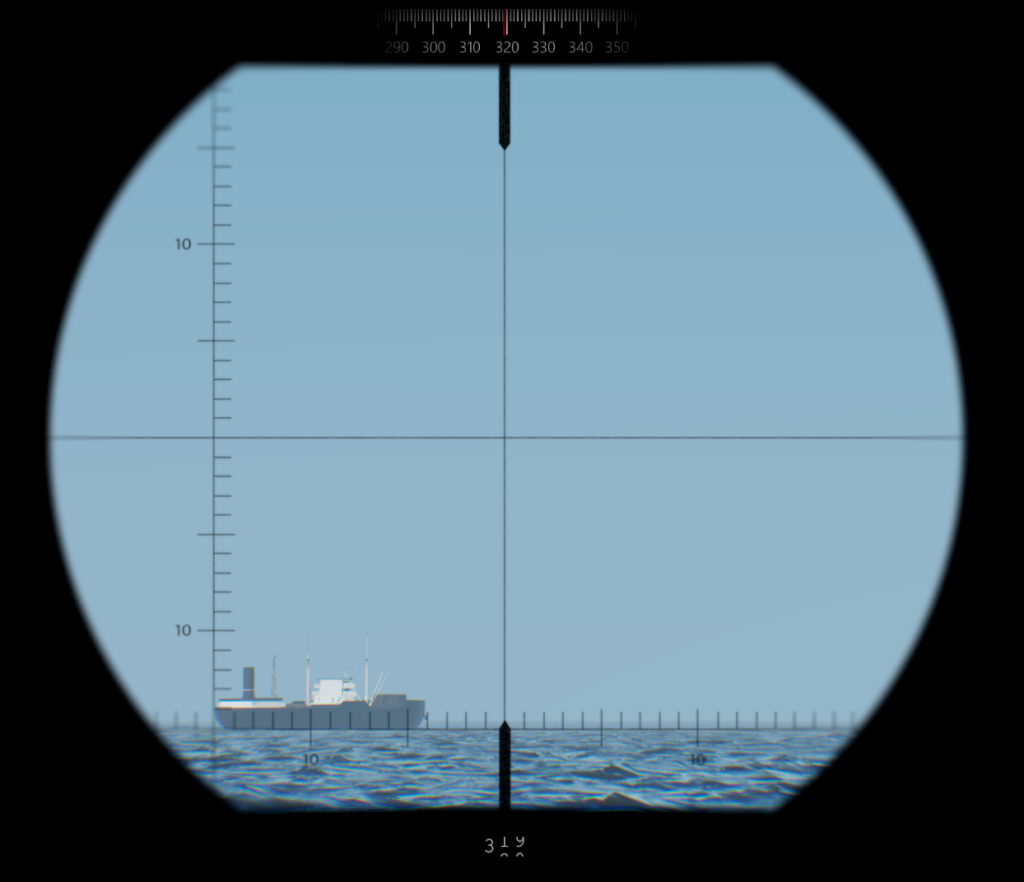
So the only quantity which needs to be measured with the periscope to deterine the angle on bow is the percieved length. This can be done by

(19) $\begin{equation*} p = \dfrac{b_h}{b_v} h \end{equation*}$

where $b_h$ is the horizontal size of the target in periscope bars, $b_v$ the vertical size of the target in periscope bars and $h$ the mast height of the target known by correct indentification. The uncertainty is

(20) $\begin{equation*} \sigma_p = \sqrt{\left( \dfrac{h}{b_v} \sigma_{b_h} \right)^2 + \left( \dfrac{b_h h}{b_v^2} \sigma_{b_v} \right)^2} \end{equation*}$

if we assume $\sigma_{b_h}$ and $\sigma_{b_v}$ are uncorrelated which is definitely not true (some positive correlation because of the change of distance of the target), but we will neglect this for now.
The next step is the sanitization of $p$

(21) $\begin{equation*} p = \begin{cases} b, & \text{if } p < b\\ \sqrt{l^2+b^2}, & \text{if } p > \sqrt{l^2 + b^2} \\ p, & \text{if } b \le p \le \sqrt{l^2 + b^2}\\ \end{cases} \end{equation*}$

and the computation of $\alpha$ . The observer must decide which $\alpha$ is more appropriate.

(22) $\begin{equation*} \alpha_1 = \begin{cases} \arctan \left(\dfrac{-lb + p\sqrt{l^2 + b^2 - p^2}}{l^2-p^2} \right), & \text{if } p \neq l \\ \arctan \left( \dfrac{l^2-b^2}{2lb} \right), & \text{if } p = l\\ \end{equation*}$

(23) $\begin{equation*} \alpha_2 = \begin{cases} \arctan \left(\dfrac{-lb - p\sqrt{l^2 + b^2 - p^2}}{l^2-p^2} \right), & \text{if } p \neq l \\ \pi/2, & \text{if } p = l\\ \end{equation*}$

The uncertainty is

(24) $\begin{equation*} \sigma_{\alpha} = \min \left( \dfrac{\sigma_p}{\sqrt{l^2+b^2-p^2}}, \sigma_{\alpha max} \right) \end{equation*}$

where $\sigma_{\alpha max}$ is a fixed maximum uncertainty.

Distance

As luck would have it the computation of distance is more straight forward.

(25) $\begin{equation*} d = \dfrac{h}{b_v} c \end{equation*}$

where $h$ is the mast height of the ship, $b_v$ the vertical size in bars of the ship in the periscope and $c$ a constant that needs to be determined based on the periscope and its zoom setting.
The uncertainty is

(26) $\begin{equation*} \sigma_d = \dfrac{h}{b_v^2} c \sigma_{b_v} \end{equation*}$

Velocity

The basic idea for a fast velocity measurement method is to let pass a certain time and count how many $b_v$ , hence horizontal bars in the periscope the target traversed. Since we measure the velocity via the periscope it makes sense to switch to an eukledian coordinate system which has $ê_x$ parallel to $b_h$ and $ê_y$ parallel to the distance vector to the target.

$\alpha$ is the angle on bow, $\beta$ the periscope heading, $v_o$ the velocity of the observer and $v_t$ the velocity of the target. With the periscope we can only measure the $ê_x$ component of $\vv{\bm{v_t}}$ . To find the absolute speed of the target we first need to isolate the effect of the movment of the observer

(27) $\begin{equation*} ê_x \cdot \vv{\bm{v_o}} = \sin(\beta) v_o \end{equation*}$

and

(28) $\begin{equation*} v_{tp} = \dfrac{b_{ht}h}{b_v t} \end{equation*}$

where $t$ is the time required to travel $b_{ht}$ horizontal bars in the periscope and $v_{tp}$ is the velocity of the target in the periscope
In order to get the absolut velocity of the target in $ê_x$ direction we just need to add both components

(29) $\begin{equation*} ê_x \cdot \vv{\bm{v_t}} = \sin(\beta) v_o + \dfrac{b_{ht}h}{b_v t} \end{equation*}$

and the total target velocity $v_t$ is

(30) $\begin{equation*} v_t = \dfrac{ê_x \cdot \vv{\bm{v_t}}}{\cos(\alpha)} = \dfrac{\sin(\beta) v_o + \frac{b_{ht}h}{b_v t}}{\cos(\alpha)} \end{equation*}$

The uncertainty of $v_t$ is dependend on quiet a lot of variables so the formula gets quiet long

(31) $\begin{multline*} \sigma_{v_t}^2 =\left( \dfrac{\cos(\beta) v_o}{\cos(\alpha)} \sigma_{\beta} \right)^2 + \left( \dfrac{\sin(\beta)}{\cos(\alpha)} \sigma_{v_o} \right) ^ 2 + \left( \dfrac{\sin(\beta) v_o + \frac{b_{ht} h}{b_v t} }{\cos(\alpha)} \tan(\alpha) \sigma_{\alpha} \right)^2 \\ + \left( \dfrac{b_{ht} h}{b_v^2 t \cos(\alpha)} \sigma_{b_v} \right) ^2 + \left( \dfrac{b_{ht} h}{b_v t^2 \cos(\alpha)} \sigma_t \right)^2 \end{multline*}$

This formula is not quiet correct since $\sigma_{\alpha}$ correlates with $\sigma_{b_v}$ but at this point I simply assumed the effects are negligible.

Closest approach and optimal intercept course

Since all relevant data of the target is available now we can add some further features. We can define a cartesian coordinate system with $ê_x$ parallel to the heading of the observer and $ê_y$ perpendicular to it.

The time depended position vector of the observer

(32) $\begin{equation*} \vv{\bm{x_o}} = \begin{pmatrix} v_o t \\ 0 \end{pmatrix} \end{equation*}$

and of the target

(33) $\begin{equation*} \vv{\bm{x_t}} = \begin{pmatrix} d_0 \cos(\beta) + v_t \cos(\alpha + \beta) t \\ d_0 \sin(\beta) + v_t \sin(\alpha + \beta) t \end{pmatrix} \end{equation*}$

can be expressed this way. The distance is

(34) $\begin{multline*} d(t)^2 = ||\vv{\bm{x_t}} - \vv{\bm{x_o}}||^2 = d_0^2 \cos(\beta)^2 + v_t^2 t^2 \cos(\alpha + \beta) + v_o^2 t^2 \\ + 2d_0 v_t t \cos(\beta) \cos(\alpha + \beta) - 2d_0 \cos(\beta) v_o t - 2v_t v_o t^2 \cos(\alpha +\beta) \\ + d_0^2 \sin(\beta)^2 + v_t^2 t^2 \sin(\alpha + \beta) + 2d_0 v_t t \sin(\alpha +\beta) \sin(\beta) \\ = d_0^2 + v_t^2 t^2 + v_o^2 t^2 + 2d_0 v_t t(\cos(\beta) \cos(\alpha + \beta) + \sin(\beta) \sin(\alpha + \beta)) \\ - 2d_0 v_o t \cos(\beta) - 2v_t v_o t^2 \cos(\alpha + \beta) \\ = d_0^2 + v_t^2 t^2 + v_o^2 t^2 + 2d_0 v_t t \cos(\alpha) - 2d_0 v_o t \cos(\beta) - 2v_t v_o t^2 \cos(\alpha + \beta) \end{multline*}$

To get the closest approach for a set $\alpha$ and $\beta$ we simply derive $d(t)$ by $t$ to find the minimum of $d(t)$ at $t_{min}$ .

(35) $\begin{equation*} \dfrac{\partial d(t)}{\partial t} = (v_t^2 + v_o^2 - 2v_t v_o \cos(\alpha + \beta)) t + d_0 (v_t \cos(\alpha) - v_o \cos(\beta)) \end{equation*}$

At the minimum this partial derivative is 0, hence

(36) $\begin{equation*} t_{min} = \dfrac{d_0 (v_o \cos(\beta) - v_t \cos(\alpha))}{v_t^2 + v_o^2 - 2 v_t v_o \cos(\alpha + \beta)} \end{equation*}$

and

(37) $\begin{equation*} d_{min} = d(t_{min}) \end{equation*}$

To derive this equation we could have also used the geometric method. At the closest approach the velocity vector is orthogonal on the distance vector.

(38) $\begin{equation*} \vv{\bm{d(t)}} = \vv{\bm{x_t}} - \vv{\bm{x_o}} \end{equation*}$

(39) $\begin{equation*} \vv{\bm{v(t)}} = \dfrac{\partial \vv{\bm{x_t}} }{\partial t} - \dfrac{\partial \vv{\bm{x_o}}}{\partial t} = \begin{pmatrix} v_t \cos(\alpha + \beta) - v_o \\ v_t \sin(\alpha + \beta) \end{pmatrix} \end{equation*}$

The dot product

(40) $\begin{equation*} \vv{\bm{d(t)}} \cdot \vv{\bm{v(t)}} = 0 \end{equation*}$

is simply 0 and we obtain the same formula for $t_{min}$ .

If we want to optimize $\beta$ to find the optimal intercept course we get a two dimensional function $d(t, \beta)$ and also need the partial derivative by $\beta$

(41) $\begin{equation*} \dfrac{\partial d(t, \beta)}{\partial \beta} = d_0 v_o t \sin(\beta) +v_t v_o t^2 \sin(\alpha +\beta) \end{equation*}$

For $t \ne 0$ , $\sin(\beta) \ne 0$ and $v_o \ne 0$

(42) $\begin{equation*} \beta = \arctan \left( \dfrac{-\sin(\alpha)}{\frac{d_0}{v_t t} + \cos(\alpha)} \right) \end{equation*}$

. Unfortunately there is no analytical way to solve $t$ and $\beta$ with equation (36) and (42)

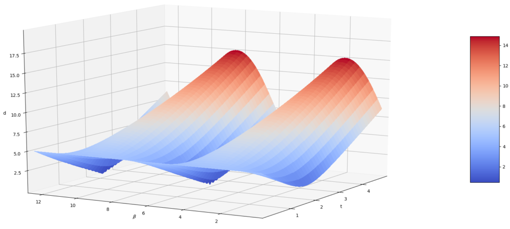3D plot of the distance in function of $t$ and $\beta$ .

The distance function has clearly a $2 \pi$ periodicity in the $\beta$ direction. The mimimum it self looks quiet well behaved without any local minimum traps and the gradient basically always points towards the minimum which should make a numerical optimization quiet effective. To speed it up we can define the gradient and Hessian matrix and use $d^2$ to get rid of taking square roots.

(43) $\begin{equation*} d(t, \beta)^2 = d_0^2 + v_t^2 t^2 + v_o^2 t^2 + 2d_0 v_t t \cos(\alpha) - 2d_0 v_o t \cos(\beta) - 2v_t v_o t^2 \cos(\alpha + \beta) \end{equation*}$

(44) $\begin{equation*} \nabla d^2 = \begin{pmatrix}(v_t^2 + v_o^2 - 2v_t v_o \cos(\alpha + \beta)) t + d_0 (v_t \cos(\alpha) - v_o \cos(\beta)) \\ d_0 v_o t \sin(\beta) +v_t v_o t^2 \sin(\alpha +\beta) \end{pmatrix} \end{equation*}$

(45) $\begin{equation*} H_{d^2} = \begin{pmatrix}v_t^2 + v_o^2 - 2v_t v_o \cos(\alpha + \beta) & 2 v_t v_o t \sin(\alpha + \beta) + d_0 v_o \sin(\beta) \\ 2 v_t v_o t \sin(\alpha + \beta) + d_0 v_o \sin(\beta) & d_0 v_o t \cos(\beta) +v_t v_o t^2 \cos(\alpha +\beta) \end{pmatrix} \end{equation*}$

This is obviously far more computationally intensive than a simple analytic formula. Luckily a triangle can save us if $d_{min} = 0$ .

At first this triangle does not seem to usefull since we only know the distance $d$ and the angle on bow $\alpha$ . the other legs depend on $t_{min}$ . But with the law of sines and knowing, that the ratio $\frac{v_o t}{v_t t}$ stays constant

(46) $\begin{equation*} \dfrac{v_t}{\sin(\beta)} = \dfrac{v_o}{\sin(\alpha)} \end{equation*}$

this simple equation follows.

(47) $\begin{equation*} \beta = \arcsin \left( \dfrac{v_t \sin(\alpha)}{v_o} \right) \end{equation*}$

If $|\frac{v_t \sin(\alpha)}{v_o}| > 1$ it means there is no intercept course with $d_{min} = 0$ and we need to fall back to the iterative optimization method.

Bonus: Torpedo hit probability

With (47) we can also analytically compute the optimal torpedo launch angle if we replace $v_o$ with the torpedo velocity. The launch angle is also refered to as gyro angle $\gamma$ .

(48) $\begin{equation*} \gamma = \arcsin \left( \dfrac{v_t \sin(\alpha)}{v_{torpedo}} \right) \end{equation*}$

If we plug in $v_t$ from (30)

(49) $\begin{equation*} \gamma = arcsin \left( \dfrac{\sin(\beta) v_o + \frac{b_{ht}h}{b_v t}}{v_{torpedo}} \tan(\alpha) \right) \end{equation*}$

and use (36) for the torpedo trajectory

(50) $\begin{equation*} t_{min} = \dfrac{d_0 (v_{torpedo} \cos(\gamma) - v_t \cos(\alpha))}{v_t^2 + v_{torpedo}^2 - 2 v_t v_{torpedo} \cos(\alpha + \gamma)} \end{equation*}$

we know the optimal launch angle and travel time of the torpedo.
If we compute the uncertainties $\sigma_{\gamma}$ and $\sigma_{t_{min}}$ and compare those to the approximate angular size of the target

(51) $\begin{equation*} \rho = \dfrac{p}{d} \end{equation*}$

and the maximum travel time of the torpedo $t_{max}$ we can determine the hit probability.

(52) $\begin{multline*} \sigma_{\gamma}^2 = \left( \dfrac{c \cos(\beta) v_o \tan(\alpha)}{v_{torpedo}} \sigma_{\beta} \right)^2 + \left( \dfrac{c \sin(\beta) \tan(\alpha)}{v_{torpedo}} \sigma_{v_o} \right)^2 + \left( \dfrac{c h \tan(\alpha)}{v_{torpedo} b_v t} \sigma_{b_h} \right)^2 \\ + \left( \dfrac{c b_{ht} h \tan(\alpha)}{v_{torpedo} b_v^2 t} \sigma_{b_v} \right)^2 + \left( \dfrac{c b_{ht} h \tan(\alpha)}{v_{torpedo} b_v t^2} \sigma_{t} \right)^2 + \left( \dfrac{\sin(\beta) v_o + \frac{b_{ht} h}{b_v t}}{v_{torpedo}} \dfrac{c}{\cos(\alpha)^2} \sigma_{\alpha} \right)^2 \end{multline*}$

with

(53) $\begin{equation*} c = \dfrac{1}{\sqrt{1 - \left( \frac{(\sin(\beta) v_o + \frac{b_{ht} h}{b_v t}) \tan(\alpha)}{v_{torpedo}} \right)^2}} \end{equation*}$

(54)

Angle on bow

Distance

Velocity

Closest approach and optimal intercept course

Bonus: Torpedo hit probability

Leave a Reply Cancel reply